Chi-squared test
The chi-squared test is not one test, but a group of tests which constitutes of all statistical tests which distribute as chi-squared distribution.
On this page, we also describe some of the alternative tests that don't use the chi-squared distribution.
All the tests on this page, except for the test for variance, are based on the multinomial model, and available on one calculator.
This page contains the following tests: chi-squared test for variance, chi-squared goodness of fit test (Pearson's), chi-squared test for independence/association, McNemar test, simulation test
Chi-squared test for variance (go to the calculator)
The chi-squared test for variance, checks if the known standard deviation is statistically correct (statistically significance), based on the sample standard deviation.
Assumptions
- Independent samples.
- The population has a normal distribution.
- σ0, the population standard deviation, is known.
Required sample data
Calculated based on a random sample from the entire population
- S - Sample standard deviation.
- n - Sample size.
Test statistic
| χ²= | (n-1)S2 |
| σ02 |
Example
Expected standard deviation: σ=20.
Sample size: n=7.
Sample standard deviation: S=31.
Degrees of freedom = 7 - 1 = 6.
| χ²= | (7-1)*312 | = 14.415 |
| 202 |
Since the p-value is larger than the significance level, 0.05066>0.05, you cannot reject the null assumption (H0).
Chi-squared goodness of fit test (Pearson's chi-squared test)
The chi-squared goodness of fit test run over a categorical variable and compares the sample data to the expected data based on the expected model.
Each category has an expected probability, per the expected model, or prior assumptions.
The null assumption is a multinomial model / binomial model. Using the chi-squared distribution is an approximation for the multinomial distribution/binomial distribution.
There are so many variations of the test, what test should you use?
Assumptions
- Independent samples.
- No overlap between the categories. (mutually exclusive)
- The observed sample data is frequencies, count of data.
- The expected model calculates the probability for each category, the multinomial model.
- For at least 80% of the categories, the frequency is at least 5.
- The frequency is at least 1 for each expected category.
When to use?
- Two categories, in this case, it is a liberal test, when you can take the risk that the type I error may be larger than the significance level (α).
- More than two categories, when meeting the minimum frequencies criteria, the type I error is similar to the significance level.
Required sample data
Calculated based on a random sample from the entire population
- Observed frequencies sample for each category.
- Expected probability per each category, based on an expected model or other prior assumption.
Examples: Normal distribution, equal probabilities, expected probabilities from other researches.
Test statistic
Calculate the statistics using the following frequencies
| χ2= | (Observed-Expected)2 |
| Expected |
k - the number of categories.
m - the number of estimated variables.
Degrees of freedom = k - m - 1
Example
Significance level: α=0.05.| Categories | Observed Frequency | Expected probability | Expected Frequency |
|---|---|---|---|
| Purple | 6 | 0.5 | 9.5 |
| Blue | 5 | 0.3 | 5.7 |
| Green | 8 | 0.2 | 3.8 |
| Total | 19 | 1 | 19 |
The following example doesn't meet the minimum 5 for at least 80% of the categories.
| χ²= | (6-9.5)2 | + | (5-5.7)2 | + | (8-3.8)2 | =6.018 |
| 9.5 | 5.7 | 3.8 |
Degrees of freedom = 3 - 0 - 1 = 2.
P-value = 1 - p( χ²(2) ≤ 6.018 ) = 0.04935.
Since the p-value is smaller than the significance level, 0.049<0.05, you may reject the null assumption (H0).
Goodness of fit with continuity correction
When to use?
- Use only for the case of two categories, when p is not 0.5.
- Conservative test, when need to be sure the type I error is less than the significance level (α).
- For some specific sample sizes, the mid-p generate better conservative results
Since the chi-squared distribution continuous is used to describe a discrete mode, the continuity correction is suggested.
The R function chisq.test doesn't support the continuity correction for the goodness of fit. The "correct = TRUE" has the same result as "correct = FALSE" (It is supported for the "test for independence").
You probably should consider using it only for two categories. Hence the webpage calculator limits the use of the correction for two categories.
Test statistic
The correction will not be bigger than the absolute difference: Min(|difference|,0.5).
| χ2= | (|Observed-Expected|-0.5)2 |
| Expected |
k - the number of categories.
m - the number of estimated variables.
Degrees of freedom = k - m - 1
Example
| χ²= | (|6-9.5|-0.5)2 | + | (|5-5.7|-0.5)2 | + | (|8-3.8|-0.5)2 | =6.018 |
| 9.5 | 5.7 | 3.8 |
Since the p-value is larger than the significance level, 0.1024>0.05, you cannot reject the null assumption (H0).
Multinomial model / Binomial model (go to the calculator)
All the tests on this page, except for the test for variance, are based on the multinomial model. The model includes a categorical variable with expected probabilities to get each category.
k - the number of categories.
n - sample size.
Prob - vector probabilities for each category, Prob=[p1, ... ,pk].
Obs - Observations values for each category, OBS=[x1, ... ,xk].
Xi - possible combination.
The following tests calculate the p-value - the probability to get the observation vector or more extreme vector, under the null assumption (H0) that the P vector is correct.
The binomial model is a special case of the multinomial model with two categories.
Example
Large container with balls.The null assumption: 50% purple balls, 30% blue balls, 20% green balls.
Sample: 6 purple balls, 5 blue balls, 8 green balls.
Prob = [0.5, 0.3, 0.2]
Obs = [6, 5, 8]
Sample size: n=19.
Xi: one of the following: [0, 0, 19], [0, 1, 18], [1, 1, 17], [2, 1, 16], [2, 2, 15], ... , [18, 1, 0], [19, 0, 0]
Significance level: α=0.05.
Multinomial test
This is the correct model, that is the reason it is called "exact test", unlike the approximated chi-squared tests.
But the fact that the test support an exact result doesn't say it is a better result!
| P(Obs) = P(X1=x1, ... ,Xk=xk)= | n! | p1x1...pkxk |
| x1!, ... ,xk! |
Xi - combination i of X.
P-value = Σ(P(Xi), for every i where P(Xi)≤P(Obs)
When to use?
- Use for three categories or more, or the conservative case of two categories with p equal 0.5
- For small probabilities, P in (0.1,0.05,0.01), the multinomial test support better result than the chi-squared test.
- Accurate test, except for the case of two categories
- The calculator currently runs only the binomial test, if you need the result of the multinomial test you may use the equivalent simulation results.
Example
Following the above example calculation.
P(Obs) = P(6,5,8) = 0.003394116 (R: dmultinom(x=c(6,5,8), prob = c(0.5,0.3,0.2)))
P(0,0,19)=5.24288e-14.
P(0,1,18)=1.494221e-12.
P(1,1,17)=6.723994e-11.
P(2,1,16)=1.428849e-09.
P(2,2,15)=1.714618e-08.
..........
P(18,1,0)=2.174377e-05.
P(19,0,0)=1.907349e-06.
P-value is the sum of all the probabilities that are less or equal to 0.003394116.
multinomial.test(c(6,5,8), c(0.5,0.3,0.2)) = 0.0635.
Simple example
Prob = [0.5, 0.3, 0.2]
Obs = [1, 0, 2]
P(Obs)=P(1,0,2)=0.06
Xi - one of the following: [0,0,3], [0,1,2], [1,0,2], ... ,[0,3,0].
P(0,0,3)=0.008.
P(0,1,2)=0.036.
P(1,0,2)=0.06.
P(0,2,1)=0.054.
P(2,0,1)=0.15.
P(1,1,1)=0.18.
P(2,1,0)=0.225.
P(1,2,0)=0.135.
P(3,0,0)=0.125.
P(0,3,0)=0.027.
P-value = 0.008 + 0.036 + 0.06 + 0.054 + 0.027 = 0.185
multinomial.test(c(1,0,2), c(0.5,0.3,0.2))= 0.185
Binomial test
The binomial test is a special case of the multinomial test with two categories.
x - frequency of category-1.
p - the probability of category-1.
n - total observations.
| P(X=i) = ( | n | )pi(1-p)n-i |
| i |
i = 0 to n.
Mid P -binomial test
Similar to the binomial test, except for taking half of P(X=x) instead of the full value.
i = 0 to n.
Comparison of the goodness of fit variations
Method
We run R simulation to compare the following four variations of the goodness of fit:
The goodness of fit test, the goodness of fit test with correction, multinomial test/binomial test, mid-p binomial test (only in case of two categories).
The sample size between 5 and 45, 40,000 repeats for each sample size. (a smaller repeat number has the same result)
We compare the following measurements:
- Type I error ratio: mean(p-value < alpha).
- The standard deviation of the p-value: sd(p-value).
The standard deviation is for each specific sample size, not between sample sizes.
We expect the type I error to be equal to the significance level (0.05).
Smaller type I error indicates a conservative test, and as a result a lower test power.
Larger type I error indicates a larger error than planed.
We prefer a test with a smaller p-value standard deviation.
Please notice that we use the simulation for two different goals, as a statistical test, a way to get test results (p-value), and as a way to check the type I error of each test.
General Results
- No test supports the required type I error!
Probably this is why there are so many variations to the test.
The reason is that the multinomial model is discrete.
Even when using the continuous chi-squared distribution over the discrete model, it doesn't support a continuous type I error! - The type I error fluctuates dramatically each time when increasing the sample size by one.
Two Categories results
P equal 0.5
- The binomial test and the chi-squared test with correction have the same type I error for most of the sample sizes, for a few sample sizes the chi-squared test with correction has lower type I error., Both tests are conservative and the average of the type I error is always under the significance level.
- The mid-p binomial test and the chi-squared test have the same type I error for most sample sizes, only for a few sample sizes the mid-p binomial is too conservative while the Mcnemar is too liberal.
Both tests fluctuate dramatically around the significance level (0.05), for some sample sizes the tests are too conservative and for some sample sizes the tests are too liberal.
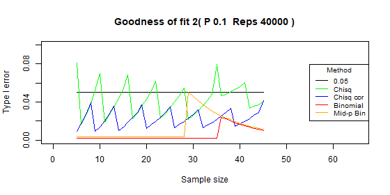
P doesn't equal 0.5 or 0.01
- Type I error
Chi-squared test - the type I error fluctuates around 0.05.
For all the other tests the type I error is always under the 0.05.
Usually: Chi-squared > Chi-squared with correction ≈ Mid-p binomial > Binomial. - Standard deviation(Type I error)
Usually: Chi-squared > Mid-p binomial > Chi-squared with correction ≥ Binomial.
Three categories results
- The multinomial test and the chi-squared test fluctuate around 0.05.
- The chi-squared test has a higher type I variance when changing the sample size.
- For a specific sample size, the chi-squared test has a lower p-value standard deviation.
Conclusions
- If possible it is better to choose the combination of sample size and test type that will support the best type I error. Hence the recommended test may be different for each combination of sample size and probability vector. The rest recommendations are only general recommendations!
- Two categories with P equal 0.5
Conservative - if you need to be sure the type I error is not bigger than the significance level, choose the chi-squared test with correction.
liberal - if you are willing to take the risk of type I error bigger than the significance level choose the chi-squared test or the mid-p binomial test. - Two categories with P other than 0.5
Conservative - if you need to be sure the type I error is not bigger than the significance level, choose the chi-squared test with correction.
Liberal - if you are willing to take the risk of type I error bigger than the significance level, choose the chi-squared test - Three categories
If the percentage of expected cells with 5 or more occurrences is at least 80%, and the value of each expected cell is at least 1, choose the chi-squared test, otherwise choose the multinomial test, or the simulation test.
Type I error - R simulation
Following the R tests we used to compare the type I error of the different variations of the goodness of fit test:
Chi squared test: chisq.test(obs, y=NULL, correct = FALSE)
Chi squared test with correction, since the R function doesn't do correction for the goodness of fit, We create the following function: chisq.test.cor
Two categories
Binomial test:
x0=min(x,n1-x)
pvalue=2*pbinom(x0, n, p). if(pvalue>1){pvalue=1}
Mid-p binomial test:
pvalue=2*pbinom(x0, n, p)-dbinom(x0, n, p)
Three categories
Multinomial test for more than 2 categories: multinomial.test(observed=obs, prob=p, useChisq = FALSE)
Two categories simulation
Following the simulation results of the goodness of fit with two categories.
The tables contain the measures , over the following sample sizes: 5-45.
Two categories - type I error: p=0.5
| Test | Average | Standard deviation | Range |
|---|---|---|---|
| Chi-squared | 0.049 | 0.016 | [0.015-0.078] |
| Chi-squared - correct | 0.029 | 0.011 | [0.001-0.048] |
| Binomial | 0.031 | 0.012 | [0.002-0.051] |
| Binomial mid-p | 0.049 | 0.015 | [0.018-0.08] |


Two categories - type I error: p=0.4
| Test | Average | Standard deviation | Range |
|---|---|---|---|
| Chi-squared | 0.048 | 0.013 | [0.01-0.087] |
| Chi-squared - correct | 0.028 | 0.01 | [0.005-0.048] |
| Binomial | 0.015 | 0.006 | [0.002-0.026] |
| Binomial mid-p | 0.026 | 0.01 | [0.003-0.054] |


Two categories - type I error: p=0.3
| Test | Average | Standard deviation | Range |
|---|---|---|---|
| Chi-squared | 0.048 | 0.015 | [0.011-0.085] |
| Chi-squared - correct | 0.027 | 0.009 | [0.003-0.043] |
| Binomial | 0.013 | 0.007 | [0.002-0.025] |
| Binomial mid-p | 0.024 | 0.011 | [0.003-0.044] |


Two categories - type I error: p=0.2
| Test | Average | Standard deviation | Range |
|---|---|---|---|
| Chi-squared | 0.044 | 0.014 | [0.017-0.073] |
| Chi-squared - correct | 0.026 | 0.009 | [0.008-0.041] |
| Binomial | 0.011 | 0.008 | [0.002-0.026] |
| Binomial mid-p | 0.021 | 0.013 | [0.003-0.047] |


Two categories - type I error: p=0.1
| Test | Average | Standard deviation | Range |
|---|---|---|---|
| Chi-squared | 0.043 | 0.016 | [0.016-0.081] |
| Chi-squared - correct | 0.022 | 0.009 | [0.009-0.042] |
| Binomial | 0.006 | 0.007 | [0.002-0.024] |
| Binomial mid-p | 0.012 | 0.014 | [0.003-0.05] |

Two categories - type I error: p=0.05
| Test | Average | Standard deviation | Range |
|---|---|---|---|
| Chi-squared | 0.043 | 0.019 | [0.019-0.102] |
| Chi-squared - correct | 0.022 | 0.010 | [0.007-0.045] |
| Binomial | 0.002 | 0.000 | [0.002-0.002] |
| Binomial mid-p | 0.003 | 0.000 | [0.003-0.003] |


Two categories - type I error: p=0.01
| Test | Average | Standard deviation | Range |
|---|---|---|---|
| Chi-squared | 0.061 | 0.038 | [0.014-0.157] |
| Chi-Squared - Correct | 0.018 | 0.014 | [0.002-0.05] |
| Binomial | 0.002 | 0 | [0.002-0.002] |
| Binomial mid-p | 0.003 | 0 | [0.003-0.003] |


Three categories simulation
Following the simulation results of the goodness of fit with three categories. The tables contain the measures , over the following sample sizes: 5-45.
Three categories - type I error: p=0.2
| Test | Average | Standard deviation | Range |
|---|---|---|---|
| Chi-squared | 0.05 | 0.005 | [0.038-0.067] |
| Chi-squared - correct | 0.024 | 0.007 | [0.008-0.033] |
| Multinomial | 0.052 | 0.004 | [0.039-0.058] |


Three categories - type I error: p=0.1
| Test | Average | Standard deviation | Range |
|---|---|---|---|
| Chi-squared | 0.051 | 0.01 | [0.028-0.088] |
| Chi-squared - correct | 0.024 | 0.005 | [0.014-0.038] |
| Multinomial | 0.049 | 0.005 | [0.03-0.055] |


Three categories - type I error: p=0.05
| Test | Average | Standard deviation | Range |
|---|---|---|---|
| Chi-squared | 0.05 | 0.009 | [0.03-0.077] |
| Chi-squared - correct | 0.025 | 0.005 | [0.01-0.034] |
| Multinomial | 0.048 | 0.003 | [0.041-0.055] |


Three categories - type I error: p=0.01
| Test | Average | Standard deviation | Range |
|---|---|---|---|
| Chi-squared | 0.07 | 0.023 | [0.038-0.131] |
| Chi-squared - correct | 0.028 | 0.013 | [0.004-0.07] |
| Multinomial | 0.047 | 0.005 | [0.033-0.056] |

Type I error - R simulation
Following the R tests we used to compare the type I error of the different variations of the goodness of fit test:
Two categories
x<-rbinom(n=1, size=n1, prob=p)
obs<-c(x,n1-x)
Chi squared test: chisq.test(obs, y=NULL, p, correct = FALSE)
Chi squared test with correction: chisq.test.cor(obs, p)
x3=min(x,n1-x)
Binomial test: pvalues3[i] <-2*pbinom(x3, n1, p)
Mid-p Binomial test: pvalues4[i] <-2*pbinom(x3, n1, p)-dbinom(x3, n1, p)
Three categories
One of the probabilities is always 0.3.
p<-c(p0,1-p0-0.3,0.3)
obs<-as.vector(rmultinom(n=1, size=n1, prob=p))
Chi squared test: chisq.test(obs, y=NULL, p, correct = FALSE)
Chi squared test with correction: chisq.test.cor(obs, p)
Since R doesn't support the correction for the goodness of fit, we create our own function: chisq.test.cor
Multinomial test: multinomial.test(observed=obs, prob=p, useChisq = FALSE)
Chi-squared test for independence/association/contingency
The Chi-squared test for independence/association is a special case of the goodness of fit test / Pearson's test.
The test compares two categorical variables.
The null assumption (H0) assumes that the two categorical variables are independent, there is no association between the variables.
The expected probability for each cell is calculated as the multiplication of the probability to get category-i in variable A and the probability to get category-j in variable B.
Assumptions
- Independent samples.
- Two categorical variables, each with no overlap between the categories. (mutually exclusive)
- The observed sample data is frequencies, count of data.
- The expected model calculates the probability for each category, the multinomial model.
- For at least 80% of the cells, the frequency is at least 5.
- The frequency is at least 1 for each expected cell.
When to use?
- Two categories, in this case, it is a liberal test, when you can take the risk that the type I error may be larger than the significance level (α), but it doesn't go dramatically above the significance level.
- When meeting the minimum frequencies criteria, the type I error is similar to the significance level.
Required sample data
Observed frequencies per each combination of the categories of both variables.
Test statistic
First, you should calculate the expected values based on the observations.
Expected P(Va=Cat-i and Vb=Cat-j) = P(Va=Cat-i)*(Vb=Cat-j).
Expected observations (Va=Cat-i and Vb=Cat-j) = P(Va=Cat-i and Vb=Cat-j) * Total observations.
The statistic is the same as the goodness of fit test:
| χ2= | (Observed-Expected)2 |
| Expected |
Degrees of freedom = (Rows-1)*(Columns-1).
Example
Two categorical variables:
- Exercise: Light, Moderate, Vigorous.
- Happiness: Not happy, Happy.
Is there an association between the level of exercise and happiness?
Observations values
| Happiness / Exercise | Light | Moderate | Vigorous | Total |
|---|---|---|---|---|
| Not Happy | 14 | 12 | 7 | 33 |
| Happy | 6 | 9 | 16 | 31 |
| Total | 20 | 21 | 23 | 64 |
Expected values
| Happiness / Exercise | Light | Moderate | Vigorous | Total |
|---|---|---|---|---|
| Not Happy | 20*33/64 | 21*33/64 | 23*33/64 | 33 |
| Happy | 20*31/64 | 21*31/64 | 23*31/64 | 31 |
| Total | 20 | 21 | 23 | 64 |
| Happiness / Exercise | Light | Moderate | Vigorous | Total |
|---|---|---|---|---|
| Not Happy | 10.31 | 10.83 | 11.86 | 33 |
| Happy | 9.69 | 10.17 | 11.14 | 31 |
| Total | 20 | 21 | 23 | 64 |
| χ²= | (14-10.31)2 | + | (12-10.83)2 | + | (7-11.86)2 | + | (6-9.69)2 | + | (9-10.17)2 | + | (16-11.14)2 | =7.095 |
| 10.31 | 10.83 | 11.86 | 9.69 | 10.17 | 11.14 |
Degrees of freedom = (2-1)*(3-1) = 2.
P-value = 1 - p( χ²(2) ≤ 7.095 ) = 0.0288. Since the p-value is smaller than the significance level, 0.0288<0.05, you can reject the null assumption (H0).
It means that there is an association between the two variables.
Association/independence model
The model is similar to the multinomial model, but the calculation of the expected probabilities is based on the multiplication of the marginal total of the two variables, and the model depends on the sampling method, with the following methods:
- Both Margins Fixed.
You plan the research to meet the required totals per each categorical variable.
In the above example, you plan the research sample to meet the exercise predefined totals:
20 - "Light" exercise.
21 - "Moderate" exercise.
23 - "Vigorous" exercise.
The same subjects should also meet the happiness predefined totals:
33 - "Not happy".
31 - "Happy". - One Margins Fixed.
You plan the research to meet the required totals per one categorical variable.
In the above example, you choose random subjects that must meet the exercise predefined totals, but you don't know what will be the distribution of the happiness categorical variable
For example, you choose subjects as following:
20 - "Light" exercise.
21 - "Moderate" exercise.
23 - "Vigorous" exercise.
But you don't know before the research, how many subjects will be "Happy" and how many "Not happy". - One Margins Fixed.
You choose a random sample and you don't know the distribution of the subjects in both categorical variables.
In the above example, you don't know before the research the exercise distribution and the happiness distribution. - Type I error ratio: mean(p-value < alpha).
- The standard deviation of the p-value: sd(p-value).
The standard deviation is for each specific sample size, not between sample sizes. - No test supports the required type I error!
Probably this is why there are so many variations to the test.
The reason is that the multinomial model is discrete.
Even when using the continuous chi-squared distribution over the discrete model, it doesn't support a continuous type I error! - The type I error fluctuates each time when increasing the sample size by one.
- When meeting the minimum frequencies criteria
The chi-Squared test support good results, fluctuates around the significance level but with a small standard deviation. The fisher test and the simulation test support similar conservative results. - When not meeting the minimum frequencies criteria,
- When meeting the minimum frequencies criteria
The chi-Squared test supports good results, fluctuates around the significance level but with a small standard deviation. The fisher test and the simulation test support similar conservative results. - When not meeting the minimum frequencies criteria, all the tests support conservative results, but the chi-squared test supports the higher type I error.
- When meeting the minimum frequencies criteria
The chi-Squared test supports good results, fluctuates around the significance level but with a very small standard deviation. The fisher test and the simulation test support similar conservative results. - When slightly not meeting the minimum frequencies criteria, all the tests support conservative results/
In extreme cases, the Fisher exact test supports the best conservative results. - 2x2 tables
Choose the chi-squared test. In some cases, it might be slightly too liberal, but I don't think it justifies using other tests. - 2x3 tables
Usually, choose the chi-squared test. In some cases, it might be slightly too liberal, but I don't think it justifies using other tests.
When you don't meet the minimum frequencies criteria, in extreme cases, it is better to use the Fisher exact test.
Comparison of association/independence variations
Method
We run R simulations to compare the following four variations of the association/independence test:
association test, association test with correction, simulation test, Fisher exact test.
The sample size between 10 and 40, 4,000 repeats for each sample size.
The generated random data is not marginal fixed. We compare the following measurements:
We expect the type I error to be equal to the significance level (0.05).
Smaller type I error indicates a conservative test, and as a result a lower test power.
Larger type I error indicates a larger error than planed.
We prefer a test with a smaller p-value standard deviation.
General Results
2x2 table results
2x3 table results
Conclusions
When the margins are not fixed.Type I error - R simulation
Following the R tests we used to compare the type I error of the different variations of the test for association of fit test:
Chi squared test: chisq.test(obs, y=NULL, correct = FALSE)
Chi squared test with correction: chisq.test(obs, y=NULL, correct = TRUE)
Simulation test: chisq.test(obs, y=NULL, simulate.p.value=TRUE, B=4000).
Fisher.test(x=obs, y = NULL,alternative = "two.sided")
2x2 Tables
Table 2x2 type I error: p=[0.2,0.2,0.3,0.3]
| Test | Average | Standard deviation | Range |
|---|---|---|---|
| Chi-squared | 0.053 | 0.006 | [0.029-0.066] |
| Chi-squared - correct | 0.017 | 0.008 | [0-0.027] |
| Simulation | 0.026 | 0.009 | [0-0.039] |
| Fisher | 0.027 | 0.01 | [0-0.042] |


Table 2x2 type I error: p=[0.1,0.3,0.15,0.45]
| Test | Average | Standard deviation | Range |
|---|---|---|---|
| Chi-squared | 0.048 | 0.007 | [0.026-0.057] |
| Chi-squared - correct | 0.011 | 0.006 | [0-0.02] |
| Simulation | 0.02 | 0.009 | [0-0.032] |
| Fisher | 0.02 | 0.009 | [0-0.033] |


Table 2x2 type I error: p=[0.05,0.35,0.075,0.525]
| Test | Average | Standard deviation | Range |
|---|---|---|---|
| Chi-squared | 0.035 | 0.008 | [0.012-0.047] |
| Chi-squared - correct | 0.005 | 0.004 | [0-0.014] |
| Simulation | 0.012 | 0.007 | [0-0.025] |
| Fisher | 0.012 | 0.008 | [0-0.025] |


Table 2x2 type I error: p=[0.01,0.39,0.015,0.585]
| Test | Average | Standard deviation | Range |
|---|---|---|---|
| Chi-squared | 0.006 | 0.002 | [0.003-0.011] |
| Chi-squared - correct | 0 | 0 | [0-0.001] |
| Simulation | 0.001 | 0.001 | [0-0.003] |
| Fisher | 0.001 | 0.001 | [0-0.003] |


2x3 Tables
Table 2x3 type I error: p=[0.2,0.08,0.12,0.3,0.12,0.18]
| Test | Average | Standard deviation | Range |
|---|---|---|---|
| Chi-squared | 0.048 | 0.006 | [0.031-0.058] |
| Simulation | 0.041 | 0.009 | [0.016-0.052] |
| Fisher | 0.041 | 0.009 | [0.019-0.052] |


Table 2x3 type I error: p=[0.1,0.18,0.12,0.15,0.27,0.18]
| Test | Average | Standard deviation | Range |
|---|---|---|---|
| Chi-squared | 0.046 | 0.003 | [0.039-0.051] |
| Simulation | 0.039 | 0.007 | [0.022-0.046] |
| Fisher | 0.039 | 0.007 | [0.023-0.046] |


Table 2x3 type I error: p=[0.05,0.23,0.12,0.075,0.345,0.18]
| Test | Average | Standard deviation | Range |
|---|---|---|---|
| Chi-squared | 0.041 | 0.006 | [0.023-0.05] |
| Simulation | 0.037 | 0.009 | [0.014-0.049] |
| Fisher | 0.038 | 0.008 | [0.019-0.051] |


Table 2x3 type I error: p=[0.01,0.27,0.12,0.015,0.405,0.18]
| Test | Average | Standard deviation | Range |
|---|---|---|---|
| Chi-squared | 0.016 | 0.005 | [0.006-0.026] |
| Simulation | 0.018 | 0.008 | [0.002-0.031] |
| Fisher | 0.03 | 0.008 | [0.006-0.04] |


McNemar test
The McNemar test is a special case of the goodness of fit test / Pearson's test.
It is a paired test for a dichotomous variable with the following values: A and B, when each subject may change the status from A to B, From B to A, or stay in the same value.
The test scope is only on the subjects that changed their status, ignoring the subjects that remain on the same status.
The null assumption (H0) is that the probability for the entire groupto change the statuses from A to B is identical to the probability to change the status from B to A, equal 0.5.
Some argue that the McNemar test doesn't look at the full model, as it looks only at the subjects that changed their status, as a result it doesn't look at the probability of a single subject to change his status.
The result of the McNemar test depends on the ratio between A and B on the "before" group, a different ratio may result in a different McNemar p-value.
An extreme example is when all the subjects are in status A, no subject will change the status from B to A.
If you choose "before" group with an identical number of subjects in status A and status B, then you may assume that the McNemar test checks the null assumption that for each subject P(A→B)=P(B→A).
| Before \ After | A | B |
| A | a: No change: | b: A to B |
| B | c: B to A | d: No change |
The result is a goodness of fit test like the following example:
| Categories | Observed Frequency | Expected probability |
|---|---|---|
| A→B: b | 12 | 0.5 |
| B→A: c | 23 | 0.5 |
Assumptions
- Independent subjects.
- No overlap between the categories. (mutually exclusive)
- The observed sample data is frequencies, count of changes.
- Equal group level probabilities to move from state A to state B and vise versa
- For at least 80% of the categories, the frequency is at least 5.
- The frequency is at least 1 for each expected category.
Required sample data
Calculated based on a random sample from the entire population
- Observed frequencies sample for each category.
- Expected probability per each category, based on an expected model or other prior assumption.
Examples: Normal distribution, equal probabilities, expected probabilities from other researches.
Test statistic
The test statistic is the same as for the goodness of., with one degree of freedom. (df = n-1 = 2-1 = 1).
| χ2= | (b - | b + c | )2+(c - | b + c | )2 |
| 2 | 2 | ||||
| b+c | |||||
| 2 |
With a basic algebra you will get the following equation.
| χ²= | (b - c)2 |
| b + c |
McNemar test with continuity correction
The McNemar test with continuity correction supports similar results to the binomial exact test, with the same characteristics:
The test is too conservative, support type I error which is smaller than the significance level.
Larger standard deviation for the p-value.
| χ²= | (|b - c| - 1)2 |
| b + c |
McNemar - binomial exact test
This is the exact calculation, supports the exact p-value, not an approximation. You may expect to get the best results, but due to the discrete characteristics of the binomial distribution, it is not possible to get type I error exactly as the significance level. The test is too conservative, support type I error which is smaller than the significance level, and larger standard deviation for the p-value.
The two-tailed test is equivalent to the chi-squared right-tailed test. Since p=0.5, the binomial distribution is symmetrical and we can calculate the two-tailed p-value as twice of the one-tailed p-values.
x=Min(b,c).
p = q = 0.5.
n = b + c.
P-value=2*P(X≤x)
| P-value=2*P(X≤x) = 2Σ( | n | )0.5i0.5n-i |
| i |
i = 0 to x.
McNemar - mid-p binomial test
This is the exact calculation, supports the exact p-value, not an approximation. You may expect to get the best results, but due to the discrete characteristics of the binomial distribution, it is not possible to get type I error exactly as the significance level. The test is too conservative, support type I error which is smaller than the significance level, and larger standard deviation for the p-value.
Comparison of McNemar variations
Since the McNemar test is a special case of the goodness of fit with two categories, the results are similar.
Method
We run R simulation to compare The following four variations of McNemar:
McNemar test, McNemar test with correction, Binomial test, Mid-p Binomial test.
The sample size between 5 and 45, 300,000 repeats for each sample size. (much smaller repeats has the same result)
We compare the following measurements:
- Type I error ratio: mean(p-value < alpha).
- The standard deviation of the type I error.
- The standard deviation of the p-value: sd(p-value).
The standard deviation is for each specific sample size, not between sample sizes.
We expect the type I error to be equal to the significance level (0.05).
Smaller type I error indicates a conservative test, and as a result a lower test power.
Larger type I error indicates a larger error than planed.
We prefer a test with a smaller p-value standard deviation.
Results
- The type I error fluctuates dramatically every time when increasing the sample size by one.
- The binomial test and the McNemar test with correction have the same type I error for most of the sample sizes, for a few sample sizes the McNemar test with correction has lower type I error.
Both tests are conservative and the average of the type I error is always under the significance level. - The Mid-p binomial test and the McNemar test have the same type I error for most sample sizes, only for a few sample sizes the Mid-p binomial is too conservative while the McNemar is too liberal. Both tests fluctuate dramatically around the significance level (0.05), for some sample sizes the tests are too conservative and for some sample sizes the tests are too liberal.
Conclusions
- If possible it is better to choose the combination of sample size and test type that will support the best type I error. Hence the recommended test may be different for each sample size (b+c).
Example: For sample size 7, all the tests generate the same type I error of 0.015, it doesn't matter which test you choose. For sample size 32, the liberal tests generate a type I error of 0.05, and the conservative tests generate 0.019, you should choose one of the liberal tests.
For sample size 43, the liberal tests generate a type I error of 0.067, and the conservative tests generate 0.019.
The rest recommendations are only general recommendations! - Conservative - if you need to be sure the type I error is not bigger than the significance level, choose the McNemar binomial.
liberal - if you are willing to take the risk of type I error bigger than the significance level chooses the McNemar test or the McNemar - mid-p binomial test.
Simulation
Following the simulation results of the McNemar test variations.
The tables contain the measures , over sample sizes: 5-45.
| Test | Average | Standard deviation | Range |
|---|---|---|---|
| McNemar | 0.049 | 0.016 | [0.015-0.078] |
| McNemar - Correct | 0.028 | 0.011 | [0-0.047] |
| Binomial | 0.029 | 0.012 | [0-0.049] |
| Binomial mid-p | 0.046 | 0.015 | [0.015-0.077] |


| Sample Size | McNemar | McNemar Correction | Binomial | Mid-p Binomial |
|---|---|---|---|---|
| 5 | 0.063 | 0.000 | 0.000 | 0.063 |
| 6 | 0.031 | 0.031 | 0.031 | 0.031 |
| 7 | 0.015 | 0.015 | 0.015 | 0.015 |
| 8 | 0.071 | 0.008 | 0.008 | 0.071 |
| 9 | 0.040 | 0.040 | 0.040 | 0.040 |
| 10 | 0.021 | 0.021 | 0.021 | 0.021 |
| 11 | 0.066 | 0.012 | 0.012 | 0.066 |
| 12 | 0.039 | 0.039 | 0.039 | 0.039 |
| 13 | 0.022 | 0.022 | 0.022 | 0.022 |
| 14 | 0.057 | 0.013 | 0.013 | 0.057 |
| 15 | 0.036 | 0.036 | 0.036 | 0.036 |
| 16 | 0.077 | 0.021 | 0.021 | 0.077 |
| 17 | 0.049 | 0.013 | 0.049 | 0.049 |
| 18 | 0.031 | 0.031 | 0.031 | 0.031 |
| 19 | 0.064 | 0.019 | 0.019 | 0.064 |
| 20 | 0.041 | 0.041 | 0.041 | 0.041 |
| 21 | 0.078 | 0.027 | 0.027 | 0.027 |
| 22 | 0.052 | 0.016 | 0.016 | 0.052 |
| 23 | 0.035 | 0.035 | 0.035 | 0.035 |
| 24 | 0.064 | 0.022 | 0.022 | 0.064 |
| 25 | 0.043 | 0.043 | 0.043 | 0.043 |
| 26 | 0.076 | 0.029 | 0.029 | 0.029 |
| 27 | 0.052 | 0.019 | 0.019 | 0.052 |
| 28 | 0.036 | 0.036 | 0.036 | 0.036 |
| 29 | 0.062 | 0.024 | 0.024 | 0.062 |
| 30 | 0.043 | 0.043 | 0.043 | 0.043 |
| 31 | 0.071 | 0.030 | 0.030 | 0.030 |
| 32 | 0.050 | 0.019 | 0.019 | 0.050 |
| 33 | 0.035 | 0.035 | 0.035 | 0.035 |
| 34 | 0.057 | 0.024 | 0.024 | 0.057 |
| 35 | 0.041 | 0.041 | 0.041 | 0.041 |
| 36 | 0.066 | 0.029 | 0.029 | 0.066 |
| 37 | 0.047 | 0.047 | 0.047 | 0.047 |
| 38 | 0.034 | 0.034 | 0.034 | 0.034 |
| 39 | 0.053 | 0.023 | 0.023 | 0.053 |
| 40 | 0.039 | 0.039 | 0.039 | 0.039 |
| 41 | 0.060 | 0.028 | 0.028 | 0.060 |
| 42 | 0.044 | 0.044 | 0.044 | 0.044 |
| 43 | 0.067 | 0.032 | 0.032 | 0.067 |
| 44 | 0.049 | 0.022 | 0.049 | 0.049 |
| 45 | 0.036 | 0.036 | 0.036 | 0.036 |
| Average | 0.049 | 0.028 | 0.029 | 0.046 |
Simulation test
The calculator also runs the Monte Carlo simulation for the multinomial model / binomial model, It runs similarly to the "simulate.p.value = TRUE" in chisq.test R function.
We use the simulation test for all the multinomial model tests (Goodness of fit/Independence/McNemar).
Bottom line:
- The simulation test is equivalent to the multinomial test or to the binomial test.
The calculator currently runs only the binomial test, if you need the result of the multinomial test you may use the simulation results. - More repeats will increase the result accuracy.
- Since the test is random, each run had a slightly different result.
- It uses the same statistics as the chi-squared test, to indicate what is a more extreme case.
- The test doesn't use the continuity correction, as there is nothing to correct. the simulation results are not continuous.
Method
Simulate the model, and check the number of random samples that are likely to happen as the observations, or less likely to happen.
The simulation test uses the same statistic as the goodness of fit test.
| χ2obs= | (Observed-Expected)2 |
| Expected | |
| χ2sample= | (Sampled-Expected)2 |
| Expected |
Calculate χ2obs statistic for the observation.
Repeat the following per the number of repeats you defined:
- Take a Random sampling of [x1, ... ,xk] from the multinomial distribution.
- Calculate the χ2sample based on the sample data
- Count when χ2sample≥χ2obs
The p-value is the ratio of the cases that are as extreme as the observations when χ2sample≥χ2obs.
Results
The results are almost identical to the exact multinomial test.
Questions
- Why the binomial exact test doesn't support the correct type I error?
Since the model is discrete model, it supports a discrete type I error, hence the type I error won't be equal to the significance level. (unless you choose significance level that falls exactly on the discrete value.)
For example Bin(n=20,p=0.5):
For X=5, p(x≤5)=0.0207, p-value=2*0.0207=0.041.
For X=6, p(x≤6)=0.0577, p-value=2*0.0577=0.1154.
The exact model is correct, but can't give you the required type 1 error, 0.05.
Any significance level between 0.041 and 0.1153 will support exactly the same type I error!. - Why the binomial exact and the chi-squared test with correction usually support exactly the same result?
The chi-squared test with correction approximates well the binomial distribution, but why exactly the same result?
Since the model is discrete, a small difference between the chi-squared distribution and the binomial distribution will have the same result: rejection or acceptance.
Example:
McNemar (16,7): exact p-value:0.0932, Chi-squared with correction:0.0953, result: accept H0.
McNemar (17,6): exact p-value:0.0346, Chi-squared with correction:0.0371, result: reject H0.
As you can see despite the difference between 0.0932 and 0.0953, and the difference between 0.0346 and 0.0371, the results are the same!
Only when the discrete result is around the significance level then you can see a large difference between the two methods, for example when n=17:
McNemar (13,4): Exact p-value: 0.0489, Chi-squared with correction: 0.0523.
Exact result: reject H0, Chi-squared result: accept H0.