Information
The following statistical tests compare the shape of the distribution to the symmetric normal distribution. The skewness test checks the level of symmetry, the kurtosis test checks how the data is spread between the tails and the middle, and the D'Agostino-Pearson test combines the two, which is what makes it a normality test.
D'Agostino-Pearson test
The D'Agostino-Pearson test checks whether the shape of the distribution is similar to the shape of the normal distribution. It is a combination of the skewness test and the kurtosis test.
It is not the most powerful normality test, but you may use it for any distribution. For a normality test, if the data does not have repeated values we recommend the Shapiro-Wilk test. If the data contains repeated values we recommend the D'Agostino-Pearson test.
Target
Tests whether the distribution model fits the observations. The tool combines the following methods:
1. A formal normality test: D'Agostino-Pearson test.
2. Graphical methods: Q-Q plot and histogram.
Skewness test
The skewness test tests the null assumption that the data distribution is symmetric, using the D'Agostino (1970) transform of √b1.
Kurtosis test
The kurtosis test tests the null assumption that the excess kurtosis equals zero, i.e. that the tails match the normal distribution's, using the Anscombe–Glynn (1983) transform of b2.
The following cards change when you change the test or the tail.
Which tail does each test use?
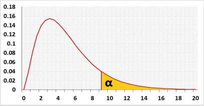
The omnibus test is right-tailed on χ²(2). That is not a contradiction with it being a two-sided question: squaring Zskewness and Zkurtosis already folds long-left and long-right tails, and heavy and thin tails, into that single upper tail, so one-sided arithmetic detects departures in either direction.
The skewness and kurtosis tests are two-tailed by default, which is what fBasics::dagoTest() reports — it offers no tail choice at all. Choosing Left or Right runs them one-tailed, matching moments::agostino.test() and moments::anscombe.test(). Note that the moments package names its tails the opposite way round from what they test: alternative = "less" gives the upper tail (positive skew / heavy tails) and "greater" the lower one. The R code this page generates already accounts for that.
Which statistics are tested?
All three tests are computed from the type 1 (population) moment ratios √b1 = m3/m21.5 and b2 = m4/m22, because the D'Agostino and Anscombe–Glynn transformations are calibrated on those. Those are the values shown in the results table. Excel's SKEW/KURT, SPSS, SAS and MINITAB each report a different sample-size correction of the same quantity — if you need to match one of those, use the skewness and kurtosis calculator, which reports all three estimators.
The tests need at least 8 observations and are unreliable below about 20.
Normality effect size
There is no single agreed effect size for a normality test. We use φ = √(χ²/n) for the omnibus test, and the sample √b1 or g2 for the two component tests. We know only the sample effect size. The effect level is a rough rule of thumb only — we still recommend looking at the Q-Q plot.
How to use this calculator
- Pick the test: the D'Agostino-Pearson omnibus, or the skewness or kurtosis component on its own.
- Type or paste one column of numbers into the grid, or use Import for a .csv or .xlsx file.
- Set the significance level (α), and the tail if you are running a component test.
- Optionally open More options to exclude outliers, change the rounding or change the histogram binning rule.
- Press Calculate.
References
- D'Agostino, R. B., Belanger, A., & D'Agostino Jr, R. B. (1990). A suggestion for using powerful and informative tests of normality. The American Statistician, 44(4), 316-321.
- D'Agostino, R. B. (1970). Transformation to normality of the null distribution of g1. Biometrika, 57(3), 679-681.
- Anscombe, F. J., & Glynn, W. J. (1983). Distribution of the kurtosis statistic b2 for normal samples. Biometrika, 70(1), 227-234.